Production, Entry, & Exit

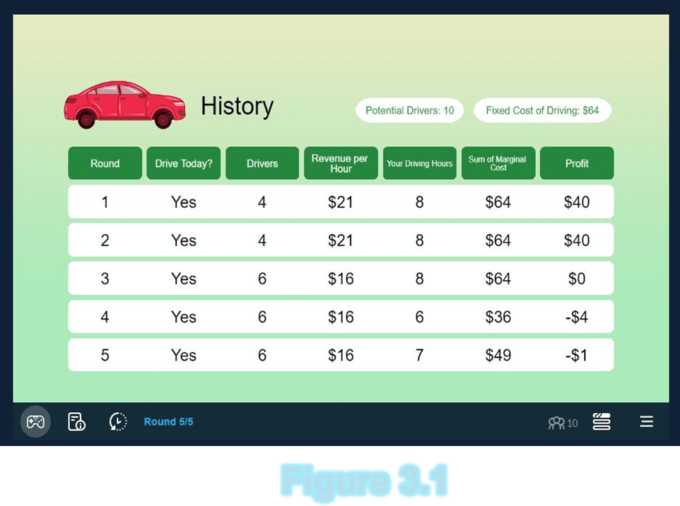
In this section, we will discuss decision-making regarding whether to enter a market, how business owners apply the concept of marginal cost to decide how much to produce, and Fixed costs changing production decisions in the short and long run using the ATC Model Figure 3.1. When I imagine owning a business, based on the simulation of being a taxi driver. The factors determining my entry and exit into this market would be understanding the many parts of my market such as Estimated Revenue Per Hour and the competition versus fixed cost and potential competition. I estimated my revenue per hour based on how many drivers. These drivers are my competitors, who drive my price down by flooding the market. Even though this allowed me to get more customers than my competitors it made me very little to no profit when my price was a low hourly wage. However, estimating drivers and hourly wages seemed hard because I needed to understand the market and I did not. So, my estimations were off a lot on whether I should or shouldn’t enter the market. As seen in Figure 3.1 I made a profit of forty dollars in the first two rounds. But the third round got me, I wasn’t paying attention to the hourly wage change, so I broke even once. When I entered the market in the last two rounds when I shouldn’t have it made me go into the negative by one to four dollars, though not a huge loss in the short run, but in the long run could turn into being out of a job. To better help you understand when it is best to exit and enter a market I am providing you with words of wisdom from Dune he wrote in 2009 “As the number of firms in the market increases, the value of continuing in the market and the value of entering the market both decline, the probability of exit rises, and the probability of entry declines… These outcomes also differ substantially across markets due to differences in exogenous cost and demand factors.”
We must identify the concept that Marginal Cost plays in deciding how much to produce. But first, we need to understand some key vocabulary. Marginal Cost is a change in cost within a given point, the output. Marginal Revenue is how the revenue changes based on output. Dealing with Marginal Cost I wanted to either break even or make a profit but always considered what that would look like before planning on how much to produce. The marginal costs varied throughout the game but the other Factors such as Fixed Cost remained the same. However, in the game, I did take two rounds to see what would happen when marginal costs were high and the hourly wage was low. Compared to what I was getting before. Both times this gave me a negative profit. Fixed Costs don’t change, that’s why they are called fixed. On the other hand, Variable Costs change in the amount of output. The marginal cost was usually quite large, so getting a low hourly wage made giving taxi rides harder because there was no profit in it.

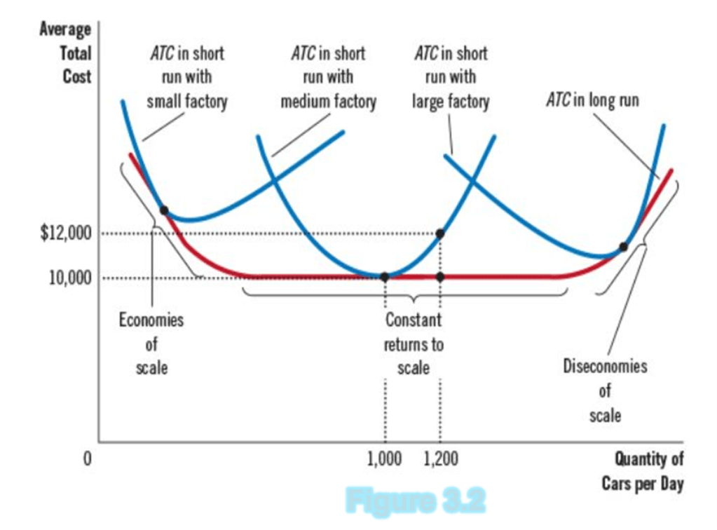
In the Long Run, there are no fixed factors, all variable factors But in the Short Run, there are both fixed and variable factors. In the long run, there are no fixed costs so the costs do not influence production. However, in the short run, there are fixed costs that influence production. For Example, looking at Figure 3.2, we can see that the average total cost is on the Y-axis and the X-axis is the quantity of Cars per day. Each blue curve represents different factory sizes in the short run, starting from the left and moving to the right with Small, then Medium, and lastly Large. The red curve represents the long-run Average total cost vs quantity produced for all factory sizes. To understand graph Figure 3.2, we must first distinguish 3 parts of the graph Economics of scale, constant returns to scale, and diseconomies of scale. Constant returns to scale are when the cost does not change regardless of output, allowing for production changes without penalty. At this stage Market changes do not affect the quantity produced. Diseconomies of scale are shown on the right side of each curve as a cost disadvantage due to increasing cost as production output increases. Economies of scale are on the left side of each curve showing the cost of production is high and production is low but is lowering to an equilibrium state where the cost and quantity of production are economical. The size of the factory changes the production rate because the business can only produce so much in the square footage of the shop floor. Keep in mind, the larger the space the higher the Average Total Cost but more can be produced. On the other hand, a smaller place has a lower Average Total Cost but less produced. We covered several key terms and their factors for production, entry and exit, Marginal cost and revenue, long run, short run, and market equilibrium.